4. Recovering An Intervention From Observation
In the previous chapter we had changed the causal graph.
Before intervention it was:
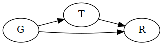
When setting $do(T=1),$ the arrow from general health into treatment was removed:
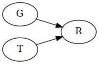
But our records came from the first situation, not the second.
Can we use them to work out what recovery would look like in the modified graph?
What The Intervention Changes
In the hospital records, treatment depended partly on general health.
That gave us a treated group consisting of 10 patients in good condition and 40 in poor condition. The untreated group had the opposite mixture: 40 in good condition and 10 in poor condition.
Under the intervention, this changes. $Do(T=1)$ means that treatment is assigned to everyone by intervention. General health no longer helps determine who receives it.
But the intervention does not change the patients' general health. Our model still contains:
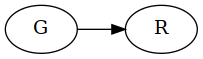
And the population still consists of 50 patients in good condition and 50 in poor condition.
So the group produced by $do(T=1)$ would have a very different health composition from the treated group in our records.
That is why:
$$ P(R\mid T=1)=0.5 $$
cannot simply be used as:
$$ P(R\mid do(T=1)). $$
Comparing Patients With The Same General Health
The observed treated group contains mostly patients in poor health. The intervention group would contain the original population mixture.
Look first only at patients in good general health.
Among them:
$$ P(R\mid T \land G)=0.9, $$
while:
$$ P(R\mid\neg T \land G)=0.8. $$
Within this comparison, general health is the same on both sides.
Now look only at patients in poor general health:
$$ P(R\mid T \land \neg G)=0.4, $$
while:
$$ P(R\mid\neg T \land \neg G)=0.2. $$
Again, general health is the same within the comparison.
Why does that help?
The problem in the aggregate comparison came from this path:
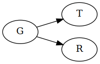
General health helped determine treatment, and it also affected recovery.
Within each health group, treated and untreated patients have the same value of $G$. Their different recovery rates cannot come from one group containing healthier patients than the other.
In our small causal model, general health is the only variable that affects both treatment and recovery.
So within each health group, the observed treatment comparison is no longer mixed with differences in general health.
We can use those rates to reconstruct what would happen if treatment were assigned independently of general health.
Reconstructing The Intervention
Imagine the 100 patients again.
Under:
$$ do(T=1), $$
all 100 receive treatment.
The intervention does not change their general-health status, so 50 are still in good condition and 50 in poor condition.
For the 50 patients in good condition, our model lets us use the observed treated recovery rate:
$$ 0.9. $$
For the 50 patients in poor condition:
$$ 0.4. $$
So the expected number of recoveries is:
$$ 50\cdot0.9+50\cdot0.4=65. $$
Across all 100 patients:
$$ P(R\mid do(T=1))=0.65. $$
Now imagine assigning no treatment to the same population.
The health distribution again remains 50 good and 50 poor.
Using the corresponding observed rates gives:
$$ 50\cdot0.8+50\cdot0.2=50. $$
So:
$$ P(R\mid do(T=0))=0.5. $$
Under the causal model we have supplied, assigning treatment raises the recovery rate from $0.5$ to $0.65$.
That is the opposite direction from the raw observational comparison:
$$ P(R\mid T)=0.5 $$
against:
$$ P(R\mid\neg T)=0.68. $$
Adjustment
What we have just done is a simple case of adjustment.
We separated the population by general health, used the treatment comparison within each health group, and then rebuilt the intervention population using the original distribution of general health.
In proportions, the treatment calculation was:
$$ 0.5\cdot0.9+0.5\cdot0.4=0.65. $$
More generally, when a variable $Z$ is appropriate for this adjustment, the same procedure can be written:
$$ P(Y\mid do(X=x)) =\sum_z P(Y\mid X=x \land Z=z)P(Z=z). $$
For each value of $Z$, take the corresponding conditional outcome probability and weight it by how common that value of $Z$ is in the population. The formula compresses the finite reconstruction. The graph tells us how to reconstruct:
General health created the path that made the aggregate treatment groups different in a causally relevant way.
Holding $G$ fixed blocked that path.
Intuitively, this works because within each health group, general health no longer varies between the treated and untreated patients. Its effect on recovery is still present, but it is no longer mixed into the treatment comparison.
We then put the health groups back together according to how common they are in the population. The influence of general health is still there, but it is now carried through the population mixture rather than through different treatment groups.
Chapter 2 already showed why this cannot become a general instruction to condition on another variable.
If the variable lies on a route through which treatment affects recovery:

Holding $B$ fixed removes part of the effect we may be trying to estimate.
The probability operations can be performed in either case.
The graph tells us what they mean causally and whether they bear on the intervention question.
What The Reconstruction Shows
We began with observational records that seemed to point in the opposite direction from the intervention result. The causal graph gave us a reason to organize those records differently for the question we were asking.
Once the graph, the recovery rates within the health groups, and the population distribution of general health remain fixed, the result is no longer independently open. Another intervention probability would require something in the graph, the observed rates, the population distribution, or the calculation to change. That is the constraint the reconstruction has made visible.
But its convincing force in the inquiry remains conditional. The calculation can be correct while the causal model is wrong.
We have seen all of that already several times.