3. Cards

Take a well-shuffled deck of 52 cards. Draw one card. For a single draw, the structure looks much like the die.

There are four aces among 52 cards.

If we treat every card as equally likely to occupy the first position in the shuffled deck, then:

$$ P(\text{ace})=\frac4{52}=\frac1{13}. $$

Now draw another card without returning the first.

Suppose the first card was an ace.

What is the probability that the second card is also an ace?

It cannot still be:

$$ \frac4{52}. $$

There are only 51 cards left. Only three of them are aces.

So:

$$ \frac3{51}. $$

The first draw has changed the situation in which the second draw occurs.

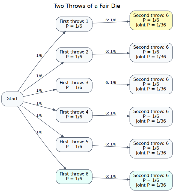
With repeated dice, the second stage presented the same six equally weighted possibilities whatever happened at the first. The deck does not.

Its later structure depends on the path already taken. That difference gives us a reason to preserve more information.

Let:

$$ A=\text{the first card is an ace} $$

and:

$$ B=\text{the second card is an ace}. $$

Before specifying what happened on the first draw, every card is equally likely to occupy the second position too, so:

$$ P(B)=\frac4{52}. $$

Given that the first card was an ace:

$$ P(B\mid A)=\frac3{51}. $$

The vertical bar preserves a difference that the changing deck has made difficult to ignore.

Consider "What is the probability that the second card is an ace?", and consider "What is the probability that the second card is an ace given that the first was an ace?"

These are very different questions. The conditions under which we evaluate event $B$ have changed. The physical deck makes the distinction easy to inspect.

A More General Multiplication Rule

We can now calculate the probability of drawing two aces.

First the first card must be an ace:

$$ P(A)=\frac4{52}. $$

Then, along that branch, the second card must also be an ace:

$$ P(B\mid A)=\frac3{51}. $$

So:

$$ P(A\land B)=P(A)P(B\mid A). $$

In this case:

$$ P(A\land B)=\frac4{52}\cdot\frac3{51}. $$

The multiplication can be reconstructed from the tree of possible events.

If we collapse some of the branches, the relevant part of the tree looks like this:

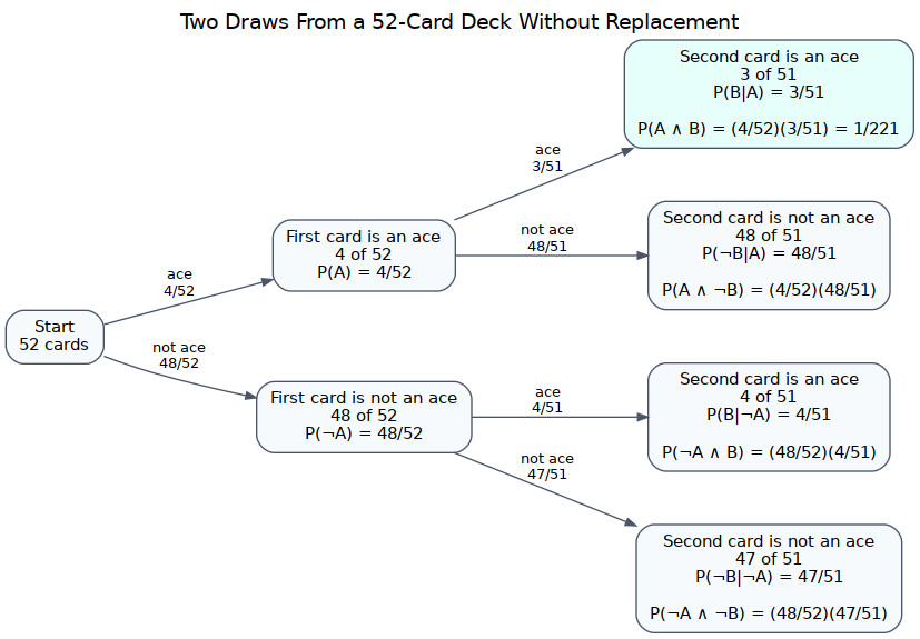
First select the $A$ branch.

Then select the part of that branch in which $B$ also occurs.

The rule we used for repeated dice now appears as a special case.

If:

$$ P(B\mid A)=P(B), $$

then:

$$ P(A\land B)=P(A)P(B). $$

The cards show us what has to remain stable for the simpler dice rule to apply: $P(B|A) = P(B)$.

In the card example, the first draw physically changes the deck. Conditional probability does not in general require one event to cause or physically alter another.

The cards are useful because they make a changing condition visible. The notation itself is more general.

From Trees To Rules

The examples with dice and cards can now be seen as two forms of the same structure.

A probability tree begins with some initial possibility and then branches further as more conditions are added.

To follow one complete path, we move stage by stage.

At each step we take the fraction that remains once the earlier stages have already been fixed.

For two stages this gives:

$$ P(A\land B)=P(A)P(B\mid A). $$

For three stages:

$$ P(A\land B\land C)=P(A)P(B\mid A)P(C\mid A\land B). $$

And similarly for longer paths.

The card example shows the more general form. The relevant fraction at the next step may depend on what happened before.

The repeated-dice case shows a special simplification. If the next-stage probabilities do not depend on what happened before, the branches no longer require different conditional weights. If the same probability also repeats at every stage, as in our repeated-die example, the product can be compressed into a power.

Independence removes the dependence of later factors on earlier outcomes. The branches can then be treated with the same weight from one stage to the next.