4. Putting The Pieces Together

Elementary Definitions

We can now define possibility spaces as finite sets.

For example the possibility space for one throw of a die is:

$$ \Omega=\{1,2,3,4,5,6\}. $$

Events are subsets of that possibility space. For example:

$$ A=\{2,4,6\} $$

is the event that the result is even, and:

$$ B=\{4,5,6\} $$

is the event that the result is greater than 3.

$$ C=\{1\} $$

is the event that the result is exactly 1.

That gives us a connection to the logic investigation that we will now look into.

There, and, or, and not operated on propositions. Here the same distinctions can operate on events.

For not, we take everything in the possibility space that does not belong to the event.

For the $A$ we defined above:

$$ \neg A=\{1,3,5\}. $$

Not even is in our case odd for the numbers in the possibility space.

More generally, for any event $A$:

$$ \neg A=\Omega\setminus A, $$

that means $\Omega$ without the elements from $A$. In other words: everything outside $A$.

The fixed possibility space matters here. It tells us what counts as everything outside $A.$

The complement of $A$ can therefore be different in a different possibility space, even when $A$ itself is the same set.

For and, we keep only the outcomes that belong to both events connected by and.

With:

$$ A=\{2,4,6\}, $$

the event that the result is even, and:

$$ B=\{4,5,6\}, $$

the event that the result is greater than 3. The outcomes 4 and 6 occur in both sets. The outcome 2 belongs only to $A$, while 5 belongs only to $B$.

So:

$$ A\land B=\{4,6\}. $$

The event that the result is even and greater than 3 leaves us with 4 and 6 given this $\Omega.$

Using set notation, the same relation can be written:

$$ A\land B=A\cap B. $$

It makes no difference which event we name first:

$$ A\land B=B\land A. $$

Both expressions select exactly the same elementary outcomes.

For or, we keep every elementary outcome belonging to at least one of the events.

Thus:

$$ A\lor B=\{2,4,5,6\}. $$

The event that the result is even or greater than 3 leaves us with 2, 4, 5 and 6 given this $\Omega.$

Using set notation, this relation can be written:

$$ A\lor B=A\cup B. $$

The outcomes 4 and 6 belong to both $A$ and $B$, but they appear only once in the combined event. We are not joining two lists. We are asking which elementary outcomes satisfy at least one of the two conditions.

Not also gives us two simple relations that will matter shortly.

No elementary outcome can belong both to $A$ and to its complement:

$$ A\land\neg A=\varnothing. $$

Together they cover the whole possibility space:

$$ A\lor\neg A=\Omega. $$

So far we have only organized possibilities.

We know which elementary outcomes belong to an event, which events overlap, and how not, and, and or change the sets under consideration.

We have constructed the structure of the events, but not yet their probabilities.

Adding Weight

Probability assigns numerical weight to these events, allowing us to distinguish between possibilities that remain open while constraining how much weight each of them can carry.

We will write that weight as:

$$ P(A). $$

In the examples so far, probabilities could often be read as shares of a whole. Three equally weighted outcomes out of six gave us:

$$ \frac{3}{6}. $$

That suggests a scale on which 0 means none of the total weight and 1 means all of it.

For the finite system we are constructing, we require three things.

First, probability weight is not negative:

$$ P(A)\geq 0. $$

An event can carry none of the available weight, but not less than none.

Second, the whole represented possibility space carries total weight 1:

$$ P(\Omega)=1. $$

The number 1 is the weight of the whole. If a finite possibility space contains $n$ elements, then:

$$ \frac{n}{n}=1. $$

That represents all of them. Assigning that weight to $\Omega$ commits the model to treating this space as exhaustive for the question it represents.

Third, consider two events that do not overlap.

Suppose $A$ contains one part of the possibility space and $B$ contains another, with no elementary outcome belonging to both:

$$ A\land B=\varnothing. $$

If probability weight represents shares of one whole, then combining two non-overlapping parts combines their shares without counting anything twice.

So we require:

$$ P(A\lor B)=P(A)+P(B). $$

The probability of events that do not overlap is additive.

Some Rules Follow

From these three requirements, several familiar probability relations follow.

Consider first the empty event.

We have:

$$ \Omega\lor\varnothing=\Omega. $$

The two sets do not overlap, so additivity gives:

$$ P(\Omega)=P(\Omega)+P(\varnothing). $$

Therefore:

$$ P(\varnothing)=0. $$

The rule for not follows in the same way.

We already know:

$$ A\land\neg A=\varnothing $$

and:

$$ A\lor\neg A=\Omega. $$

Additivity therefore gives:

$$ P(A)+P(\neg A)=P(\Omega). $$

Since:

$$ P(\Omega)=1, $$

we obtain:

$$ P(\neg A)=1-P(A). $$

So once the whole space has weight 1, the probability of not $A$ is whatever weight remains outside $A$.

Or requires one additional step when the events overlap.

For our die let again:

$$ A=\{2,4,6\} $$

and:

$$ B=\{4,5,6\}. $$

Their overlap is:

$$ A\land B=\{4,6\}. $$

If we add:

$$ P(A)+P(B), $$

the weight belonging to 4 and 6 is included twice.

So one copy of the overlap has to be removed:

$$ P(A\lor B) =P(A)+P(B)-P(A\land B). $$

For a fair die:

$$ P(A)=\frac36, $$

$$ P(B)=\frac36, $$

and:

$$ P(A\land B)=\frac26. $$

Therefore:

$$ P(A\lor B) =\frac36+\frac36-\frac26 =\frac46. $$

That agrees with the four elementary outcomes we can inspect directly:

$$ A\lor B=\{2,4,5,6\}. $$

The formula compresses the same structure.

And Needs More Information

Suppose we know:

$$ P(A) $$

and:

$$ P(B). $$

Does that determine:

$$ P(A\land B)? $$

Take a possibility space with four equally weighted elementary outcomes:

$$ \Omega=\{1,2,3,4\}. $$

Let:

$$ A=\{1,2\}. $$

Then:

$$ P(A)=\frac12. $$

Now consider three different events:

$$ B_1=\{1,2\}, $$

$$ B_2=\{1,3\}, $$

and:

$$ B_3=\{3,4\}. $$

Each has probability:

$$ \frac12. $$

But their overlaps with $A$ differ.

For $B_1$:

$$ A\land B_1=\{1,2\}, $$

so:

$$ P(A\land B_1)=\frac12. $$

For $B_2$:

$$ A\land B_2=\{1\}, $$

so:

$$ P(A\land B_2)=\frac14. $$

For $B_3$:

$$ A\land B_3=\varnothing, $$

so:

$$ P(A\land B_3)=0. $$

In every case:

$$ P(A)=P(B_i)=\frac12. $$

Knowing the separate weights of $A$ and $B$ does not tell us how much weight belongs to both.

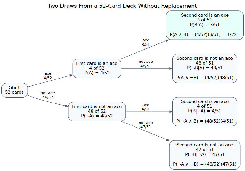
The tree from the card example shows what is missing.

To find $P(A\land B)$, we first followed the branch on which $A$ occurred. Then, within that branch, we asked what share also belonged to $B$.

That restricted share is what we wrote as:

$$ P(B\mid A). $$

And needs conditional probabilities.

Conditional Probability

The card tree gave us the missing relation.

To reach the event $A\land B$, we first follow the branch on which $A$ occurs.

That branch carries weight:

$$ P(A). $$

Once we are on that branch, we ask how likely $B$ is under the condition that $A$ has already occurred.

We write that as:

$$ P(B\mid A). $$

In the card example, this was easy to determine directly. Once the first card was known to be an ace, 51 cards remained and 3 of them were aces, so:

$$ P(B\mid A)=\frac3{51}. $$

In other problems, determining a conditional probability may be much harder. But once we have it, the tree tells us how the two stages fit together.

We take the weight of the $A$ branch and then the share of that branch in which $B$ occurs:

$$ P(A\land B) =P(A)P(B\mid A). $$

This is the more general multiplication rule we used in the previous chapter.

In the last chapter we used this visualization:

Independence

Repeated fair-die throws gave us a simpler case for and.

There, learning the result of the first throw did not change the probabilities assigned to the possible results of the second.

If $A$ and $B$ have that relation, then:

$$ P(B\mid A)=P(B). $$

We call them independent.

Substituting this into:

$$ P(A\land B) =P(A)P(B\mid A) $$

gives:

$$ P(A\land B) =P(A)P(B). $$

The multiplication rule we used for independent die throws is therefore a special case of the conditional relation.

Equal Weighting

For the fair die, we treated the six elementary outcomes as carrying equal weight.

Let the weight of each one be:

$$ w. $$

Since the six outcomes together make up the whole possibility space:

$$ 6w=1. $$

Therefore:

$$ w=\frac16. $$

For the event:

$$ A={2,4,6}, $$

additivity gives:

$$ P(A) =\frac16+\frac16+\frac16 =\frac36. $$

More generally, when the elementary outcomes in a finite possibility space are equally weighted:

$$ P(A)=\frac{|A|}{|\Omega|}. $$

Counting produces probabilities only after equal weighting has been justified.

For the fair die, its symmetry gave us a reason to assign equal weights to the six elementary outcomes.

The loaded die showed why that step matters. Six possible faces do not by themselves imply six equal probabilities.

What This Construction Shows

We can now return to the two questions about convincing force which guide the second part of this essay cycle.

The first question concerns the constraint inside the probability system.

Once $\Omega$ is fixed, the events are represented as sets of elementary outcomes. We can inspect which outcomes belong to $A$, which belong to $B$, where they overlap, and what remains outside an event.

Probability then adds weight.

We treated 1 as the weight of the whole possibility space, required weights to be non-negative, and required the weights of non-overlapping parts to add.

Once those conditions are fixed, some further relations are no longer separate choices.

If $A$ and $\neg A$ divide the whole space between them, their weights must add to 1.

If $A$ and $B$ overlap, adding their separate weights counts the overlap twice, so one copy has to be removed.

If we follow an $A$ branch and then ask for the weight of $B$ under that condition, the weight of $A\land B$ is fixed by the two stages:

$$ P(A\land B)=P(A)P(B\mid A). $$

For small enough problems, the route to those relations remains open to inspection.

We can write down the possible outcomes, group them into events, inspect overlaps, follow branches in a tree, count, and compare the formulas with the structure from which they were derived.

That is one source of the convincing force of the constraints produced by probability theory. The formulas compress relations that can still be reconstructed.

The second question concerns applying the formal system of probability to a problem.

As in logic, applying the formal system depends on prerequisites that are not usually fully under our control.

The possibility space has to contain the possibilities that matter for the question. The elementary outcomes have to represent the distinctions that matter for the question. Equal weighting, when used, needs support. A claim of independence has to fit the situation. Conditional probabilities have to be estimated or otherwise justified.

The probability calculus does not settle those questions for us.

They can be examined separately from the formal relations that follow once the inputs are fixed.

So the formal constraint may be highly convincing while its application to a particular problem remains doubtful.