5. Bayesian Updating

Winning The Lottery

You entered a lottery a few weeks ago.

One morning you receive an email saying that you have won one million euros. Click here.

At first you are suspicious. Messages like this are often scams.

But the email made it to the inbox in the first place. And the email carries the right lottery logo. The wording looks professional. That makes a genuine message seem somewhat more plausible.

Then you look at the sender.

The address is not from the lottery's usual domain. That counts against the message being genuine. But the address is not completely implausible either. Maybe they send such messages from another domain. It is still strange.

The balance shifts again. Each clue fits the two possibilities differently, but neither of them settles which possibility is true.

The setting is different from the earlier examples of cards and dice. There we worked with finite arrangements of outcomes.

Here we are comparing two hypotheses in the light of evidence: the message is genuine, or it is a scam. The weights we assign in such a setting often come from quite different sources.

The initial weights of the hypotheses may depend on background information, previous experience, base rates, or judgment.

The likelihoods require another kind of assessment: how likely would this evidence be if the message were genuine, and how likely would it be if it were a scam?

Those quantities are usually not read directly from a small finite arrangement in the way they were for dice, cards, or socks.

Many questions involve such a setup: several hypotheses remain open, their weights are not given simply by counting a finite arrangement, and new evidence bears differently on them. What is causing the strange noise in the car? Why has a plant suddenly stopped growing? Which explanation best fits an unexpected result?

In such cases, how should the weights assigned to the hypotheses change when new evidence is taken into account?

That is the problem Bayesian updating addresses.

Turning The Conditional Around

We already have:

$$ P(A\land B)=P(A)P(B\mid A). $$

From the previous chapter we also know:

$$ A\land B=B\land A. $$

So the same joint event can be reached from the other direction:

$$ P(B\land A)=P(B)P(A\mid B). $$

Since both expressions on the right side describe the same event, they must be equal to each other:

$$ P(A)P(B\mid A)=P(B)P(A\mid B). $$

If:

$$ P(B)>0, $$

we can divide by $P(B)$:

$$ P(A\mid B)=\frac{P(B\mid A)P(A)}{P(B)}. $$

That is Bayes' theorem.

Mathematically, it is an ordinary probability theorem.

Why, then, has it become so prominent?

The reason is easier to see when the conditional we know is not the conditional we want. But this is just the first step.

Bayes' Theorem

Suppose:

$$ H=\text{a person has disease D} $$

and:

$$ E=\text{a diagnostic test is positive}. $$

Imagine that in a certain population:

$$ P(H)=0.01. $$

One person in one hundred has the disease.

Suppose the test returns a positive result for 90 percent of people who have it:

$$ P(E\mid H)=0.90. $$

And suppose it also returns a positive result for 5 percent of people who do not:

$$ P(E\mid\neg H)=0.05. $$

A person tests positive.

How likely is it that the person has the disease?

The 90 percent figure is tempting.

But it answers: Given the disease is present, how likely is a positive test?

We want: Given a positive test, how likely is the disease?

Those are:

$$ P(E\mid H) $$

and:

$$ P(H\mid E). $$

They are not the same conditional.

We can answer the second question without Bayes' theorem.

Imagine 10,000 people.

About 100 have the disease.

Of those, about 90 test positive.

The other 9,900 do not have the disease.

Five percent of them also test positive:

$$ 495. $$

So there are about:

$$ 90+495=585 $$

positive tests.

Of those, about 90 come from people with the disease:

$$ P(H\mid E) \approx \frac{90}{585} \approx0.154. $$

After conditioning on the positive result, the probability in the model has moved from one percent to about fifteen percent. But it has not moved to ninety percent.

Bayes' theorem lets us calculate that result in a general way.

A positive test can occur in two mutually exclusive ways: the person has the disease and tests positive, or the person does not have the disease and tests positive.

So:

$$ P(E)=P(E\land H)+P(E\land \neg H). $$

Using the multiplication rule from the previous chapter:

$$ P(E\land H)=P(H)P(E\mid H) $$

and:

$$ P(E\land \neg H)=P(\neg H)P(E\mid\neg H). $$

Combining the two branches gives:

$$P(E)=P(E∣H)P(H)+P(E∣¬H)P(¬H).$$

So:

$$ P(E) =0.90\cdot0.01 + 0.05\cdot0.99 =0.0585. $$

We now have all the pieces we need:

The prior probability of the hypothesis:

$$ P(H)=0.01. $$

The probability of the evidence if the hypothesis is true:

$$ P(E\mid H)=0.90. $$

The total probability of the evidence:

$$ P(E) = 0.0585 $$

What we want is:

$$ P(H\mid E), $$

the probability of the hypothesis given the evidence.

We take Bayes' theorem

$$ P(H\mid E) =\frac{P(E\mid H)P(H)}{P(E)}. $$

and plug the values in:

$$ P(H\mid E) =\frac{0.90\cdot0.01}{0.0585} \approx0.154. $$

Both routes lead to the same result.

We can construct an imagined finite population and count. Or we can use the algebraic relation.

The formula reaches the same result while doing much less work.

Up to this point, we are still close to the world of dice and cards. The numbers supplied to the calculation may come from earlier observations or measurements, but the inversion itself can still be reconstructed through an explicit finite arrangement.

The situation changes when the possibilities themselves are hypotheses. That is the second step.

Between Hypotheses And Evidence

We saw that Bayes' theorem is a mathematical theorem about a relation between conditional probabilities.

In Bayesian inference, it is usually given a particular interpretation: one conditional represents how likely some evidence would be under a hypothesis, and the other represents how probable the hypothesis is given that evidence.

We begin with a set of hypotheses representing possible explanations of what is happening. Some carry more weight than others before the present evidence is taken into account. We assign probabilities to those hypotheses to represent the weight we give them.

Something we have observed that bears on our investigation becomes evidence, $E$.

The likelihood connects the two sides. For each hypothesis $H_i$, we ask how likely this particular evidence would be if that hypothesis were true.

That gives us $P(E\mid H_i).$ In many applications, this is the conditional we can estimate or model more directly.

Bayes' theorem then carries the relation in the other direction. Once $E$ has been observed, it constrains how the weights assigned to the hypotheses change, giving us $P(H_i\mid E)$.

This gives the mathematics a particular role in inquiry. We can represent explanatory hypotheses we have in mind, represent evidence we encounter, and connect them through claims about what each hypothesis would lead us to expect.

Those connecting claims are doing substantial work. If two hypotheses make $E$ equally likely, that evidence does not distinguish between them. If one makes $E$ much more likely than another, the observation shifts their relative weights, as in this schema:

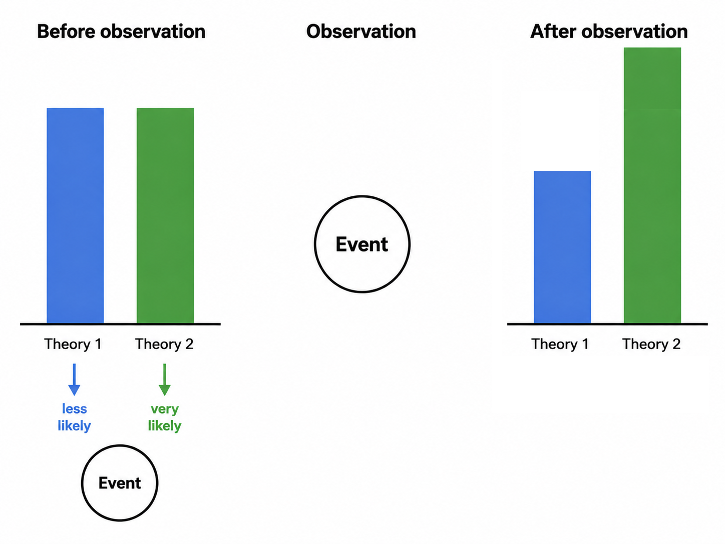
That is what gives Bayes' theorem its particular importance in Bayesian inference. An ordinary relation between conditional probabilities becomes a model for a common situation in inquiry: several hypotheses remain open, evidence bears differently on them, and their relative weights change as that evidence is taken into account.

When The Possibilities Are Hypotheses

A computer repeatedly restarts under heavy load.

Several explanations occur to us.

The power supply may be failing. The machine may be overheating. Memory could be defective.

Call these:

$$ H_1=\text{power supply failure}, $$

$$ H_2=\text{overheating}, $$

and:

$$ H_3=\text{memory failure}. $$

We observe:

$$ E=\text{the machine restarts under heavy load}. $$

We can ask:

$$ P(H_i\mid E). $$

That form is familiar. But unlike the cards in the earlier examples, the hypotheses are not given to us by an arrangement we can simply inspect. We cannot spread every possible explanation of the machine failure across a table and check that all of them are present. We have to come up with the possibilities somehow.

A technician may recognize familiar failure patterns. The age of the power supply may make one possibility salient, or overheating may have occurred before. Memory problems may also be common in similar machines.

Why exactly these three?

The operating system may contain a bug, the motherboard may be failing, the external power supply may be unstable, or two faults may occur together.

The probability model can distribute weight only among possibilities represented in it.

If an important hypothesis is missing, no flawless update can assign probability to it until the model changes.

This is the old problem of possibility generation in another form. With dice and cards, the completeness of the possibility space was easy to inspect. Here, the conviction that the relevant possibilities have been included has to come from somewhere else.

Priors

For this small model, suppose we treat these three hypotheses as mutually exclusive and exhaustive: exactly one of them is taken to explain the failure.

We assign:

$$ P(H_1)=0.50, $$

$$ P(H_2)=0.30, $$

$$ P(H_3)=0.20. $$

These are priors: the probabilities assigned to the hypotheses before (prior to) the observation $E$ is used to update them.

Where did they come from?

Comparable failures may historically have been power-supply problems about half the time. A technician might instead translate her own judgment of plausibility into numbers, or the values may come from another statistical model. These are examples of where the convincing force of a prior can come from. Its source can then itself be examined.

Likelihoods

We also need to know how expected the observation would be under each hypothesis.

Suppose:

$$ P(E\mid H_1)=0.80, $$

$$ P(E\mid H_2)=0.60, $$

$$ P(E\mid H_3)=0.20. $$

That says roughly: the evidence we are looking at is very likely under the first hypothesis, likely under the second, and not so likely under the third.

The likelihood, too, has to be convincing enough to enter the model. Whatever supports that estimate lies outside the update itself.

Likelihoods do not have to add up to 1. Each is the probability of the evidence under a different condition.

Evidence

Even $E$ had to be constructed.

Something happened in the machine.

We represented it as "The machine restarts under heavy load."

We might instead have recorded "The machine restarts within thirty seconds above 80 percent CPU load", or "The machine loses power without a kernel panic."

Those descriptions preserve different distinctions. The world does not arrive carrying an $E$ label.

Something becomes salient, is observed, classified, measured or described, and then enters the formal process in a particular representation.

That representation can change the likelihoods assigned under the hypotheses.

Once $E$ has been represented, we still need its probability.

For this model, the three hypotheses are mutually exclusive and exhaustive. Exactly one of them is taken to be true, and together their probabilities add to 1.

So if the evidence $E$ occurs, it must occur together with one of the three hypotheses:

$$ E =(E\land H_1) \cup (E\land H_2) \cup (E\land H_3). $$

These three cases do not overlap.

From the addition rule:

$$ P(E) =P(E\land H_1) + P(E\land H_2) + P(E\land H_3). $$

And from the multiplication rule:

$$ P(E\land H_i) =P(H_i)P(E\mid H_i). $$

So:

$$ P(E) =P(H_1)P(E\mid H_1) + P(H_2)P(E\mid H_2) + P(H_3)P(E\mid H_3). $$

With our values:

$$ P(E) =0.50\cdot0.80 + 0.30\cdot0.60 + 0.20\cdot0.20 =0.62. $$

More generally, suppose the model contains mutually exclusive and exhaustive hypotheses

$$ H_1,\ldots,H_n. $$

Under each hypothesis, part of the probability of the evidence comes from:

$$ P(E_i)=P(E\land H_i) =P(H_i)P(E\mid H_i). $$

The hypotheses do not overlap, so these contributions can be added. And because they exhaust the represented possibilities, there is no other part of $E$ left outside them. Thus:

$$ P(E) =P(E_1)+P(E_2)+\dots +P(E_i)= $$ $$ P(H_1)P(E\mid H_1) + P(H_2)P(E\mid H_2) + \cdots + P(H_n)P(E\mid H_n). $$

Or more compactly:

$$ P(E)=\sum_{i=1}^{n}P(H_i)P(E\mid H_i). $$

Each hypothesis contributes according to how much probability it has and how likely the evidence would be under it. Adding those non-overlapping contributions gives the full probability of the evidence.

The Update

Now suppose the model is in place.

We have:

$$ P(H_1)=0.50, \quad P(H_2)=0.30, \quad P(H_3)=0.20 $$

and:

$$ P(E\mid H_1)=0.80, \quad P(E\mid H_2)=0.60, \quad P(E\mid H_3)=0.20. $$

The probability of the observation under the model is:

$$ P(E) =0.80\cdot0.50 + 0.60\cdot0.30 + 0.20\cdot0.20. $$

So:

$$ P(E)=0.62. $$

The posterior probabilities are:

$$ P(H_1\mid E) =\frac{0.80\cdot0.50}{0.62} \approx0.645, $$

$$ P(H_2\mid E) =\frac{0.60\cdot0.30}{0.62} \approx0.290, $$

and:

$$ P(H_3\mid E) =\frac{0.20\cdot0.20}{0.62} \approx0.065. $$

What The Bayesian Investigation Shows

What makes the constraint inside Bayesian updating convincing?

Bayes' theorem was reconstructed from the multiplication rule established in the previous chapter:

$$ P(A\land B)=P(A)P(B\mid A), $$

from the fact that:

$$ A\land B=B\land A, $$

and algebra.

That gives us a route back through the formula.

We can inspect the multiplication rule, inspect why $A\land B$ and $B\land A$ describe the same event, and follow the algebraic rearrangement step by step.

The diagnostic example gave us another way to inspect the same relation.

Bayes' theorem gave us the same result from the prior and the two conditional probabilities.

In cases like this, the probabilities can be represented as proportions of finitely many equally weighted cases, so the calculation can be reconstructed by counting those cases directly.

That is not always possible exactly. Even a finite probability space can contain weights that cannot be expressed as a ratio of two finite counts.

But even then, the route back to the structure remains open. We can still lay out the elementary possibilities, assign the weights supplied by the model, and calculate the relevant conditional probabilities directly from those weighted possibilities.

It is again inspectability that lends some convincing force. In simple cases we can reconstruct it by counting. In more general finite cases we can reconstruct it from explicitly weighted possibilities and from relations whose operation has already become familiar in the simpler examples.

The hypothesis example showed the same constraint in a richer model. Once the model is fixed, the posterior values are not separately open. If one of them is to change, something else in the model has to change with it.

This differs somewhat from the logical cases. There, much of the visible constraint worked by exclusion. A possibility survived or did not. A counterexample existed or did not.

Here several hypotheses can remain open while their relative weights become constrained.

The second question concerns applying Bayesian updating to an actual problem.

As in logic, applying the formal system depends on prerequisites that are not usually fully under our control.

The hypothesis space has to contain possibilities that matter for the question. Bayes' theorem cannot assign weight to a hypothesis that never entered the model.

This returns us to the problem of possibility generation from Part I. With cards, completeness was easy to inspect. With explanations for a computer failure, it is not.

The priors also need support. Whatever their source, their convincing force has to arise outside the Bayesian update itself.

The same is true of likelihoods. A value such as $P(E\mid H_1)=0.80$ has to be convincing enough to enter the model. The update tells us what follows from that value once it is supplied.

The evidence has prerequisites of its own. The world does not arrive carrying an $E$ label. Something becomes salient, is observed, measured, classified, or described, and then enters the model in a particular representation.

Those differences can matter to the likelihoods and to the update.

There is another prerequisite as well.

The Bayesian interpretation itself has to be convincing, both as a way of relating hypotheses to evidence and as a suitable representation of this particular problem.

We have used Bayes' theorem by treating possible explanations as hypotheses that can carry probability, treating an observation as evidence, and using likelihoods to represent what each hypothesis would lead us to expect.

We then interpret conditioning on that evidence as a change in the weights of the hypotheses.

This asks more than the small finite arrangements we reconstructed earlier, because more of the formalism now has to stand for something outside the calculation.

So the convincing force of Bayesian updating depends on more than the correctness of the calculation and the support for its numerical inputs. The bridge we have built between hypotheses and evidence has to be convincing as well.

Appendix A sketches two central parts of a real Bayesian investigation: maintaining a hypothesis space, and updating the weights within it as evidence arrives.

As long as the hypothesis space remains fixed, the updating is mathematical. But as we have seen, during inquiry other possibility can come up, and the space itself then needs to change.

The appendix shows how these two moves can alternate and some of the places where their inputs can go wrong.

The Posterior Is Not The Conviction

Suppose the calculation gives:

$$ P(H_1\mid E)\approx0.645. $$

That is a result inside the model.

A technician may become more convinced that the power supply is failing.

She may also question the prior, a likelihood, the hypothesis space, the way the evidence was represented, or whether this is an appropriate model of the problem.

The posterior and the conviction are not the same thing.

The calculation can participate strongly in conviction formation without determining what the person will become convinced of.

It can also make disagreement more precise.

If the arithmetic is accepted but the posterior is not, attention can move to what the result depends on.

A prior may be challenged. A likelihood may need better support. Another hypothesis may have been omitted. The evidence may have been represented differently.

The formal structure can expose where something would have to change if the result is to change.